Chapter 4
Details of the Decision Support System Model Base
4.1 Introduction
The various mathematical, engineering models in a Decision Support System is termed as the Model Base. When the end-user starts running a module, the appropriate model is selected from the Model Base and the relevant data extracted from the Database, and the solutions to the model are either sent directly to the end user, or can serve as an input to another model in the Model Base. Models can be categorized as Strategic Models, Tactical Models, Operational Models or, Model building blocks and subroutines.
The Strategic Models are used by top management to determine the objectives of an organization, the resources needed to accomplish those objectives, and the policies to govern the acquisition, use and disposition of these resources. They may be used for company objectives planning, plant location problem, environmental impact planning, or other similar types of application. These models tend to be very broad in scope with many variables expressed in compressed aggregated form. And the data required is mainly subjective. The time horizons for these models are much longer, often in years.
The Tactical Models are commonly employed by middle management people to assist in allocating and controlling the use of the organization's resources. Applications include Financial Planing, workers' requirement planning, sales promotion planning, and plant layout determination. These models are applicable to a subset of the organization, like Production, or Marketing, or Accounting, and have some aggregation of variables. The time horizon is much lesser here, and is one or a few months. Some subjective and external data are needed, but the greatest requirements are for the internal data.
The Operational Models are usually employed to support the short-term decisions, like daily or monthly and are found in lower organizational levels. Potential applications include media selection, production scheduling, and inventory control. They are typically deterministic, and provide optimization information.
In addition to strategic, tactical, and operational models, the model base contains model building blocks and sub-routines. They include Linear Programming, time series analysis or regression analysis. They can be used separately for ad hoc decision support, or together to construct and maintain more comprehensive models.
These models when integrated together form the Model Base for a Decision Support System. In this chapter we discuss the various models that have been taken into consideration for our overall objective of optimizing the distribution of Fertilizers.
The novel features of the Model Base that we have designed are:
All the models can be categorized into anyone of the above-discussed subsystems or a conglomeration of two or more of them.
4.2 Important modules in the DSS
Figure 4.1 Major Modules in the Decision Support System
The Figure shows the various Modules that we have taken into consideration. They are directly linked to the Database and while the initial block of the model base run independently, the others are dependant on the output of models of the preceding stage or, parent model subsystem. In the later sections of this chapter, we will discuss various aspects taken into consideration in each of these modules.
4.3 The Clustering Algorithm Module
The Modes for transportation of Fertilizers are Rail and Road. Though all warehouses can be reached through road from the source points, railways are not accessible to many places. Furthermore, rakes are unloadable only at specific places, called Rake points, from which the Fertilizers have to be supplied to the non-rake point warehouse locations by road. The Clustering algorithm helps to group warehouses into Clusters. Every cluster has only one Rake point and that is called the cluster head. The clustering can be done using 1 - median algorithm in a Network.
The Clustering Algorithm is a heuristic by which the neighboring non-rake warehouses are located around a particular rake point. Factors like road distances, secondary freights are taken into consideration.
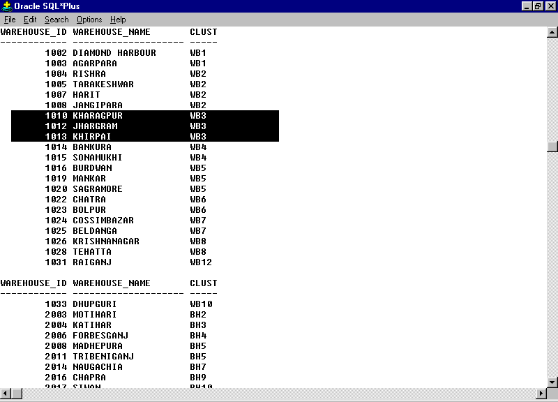
Figure 4.2 Table whouse_det
4.4 The Shortest Path Module
The shortest route (both by Railways and by Road) for reaching a particular warehouse is estimated with the help of maps, from every source point using Diskstra's Algorithm. The details of the routes and the route distances are present in the table distance.
4.5 The Customer Accounts Profitability Module
4.5.1 Customer Accounts Profitability
The Customer Accounts Profitability or, CAP, is the contribution per ton due to a supply between a source and a specific warehouse. It is a measure of the effectiveness of Fertilizers being sent from a source to a warehouse in a particular mode [Gattorna, 1992]. The CAP algorithm differs with the mode of transportation that is selected. In this section, we will discuss each one of them shortly. In all the calculations, we have a Model sheet that gets copied as Clusters are added for calculation.
4.5.2 CAP By Road
The road option as a mode of transport is feasible only when, the distances between warehouses and the source are not very long. Keeping this in mind, we have considered cases of Haldia being able to supply by road to only West Bengal clusters. We will explain the procedure in which the CAP is calculated from the screen shot of the algorithm page.
The shot below is a typical case in which the Source is Haldia, and 3 warehouses are taken into consideration. The input to this module is the Sales plan, which is taken directly from the Database. Then we calculate the Safety Stock. The empirical algorithm [Peterson and Silver, 1979] used is:
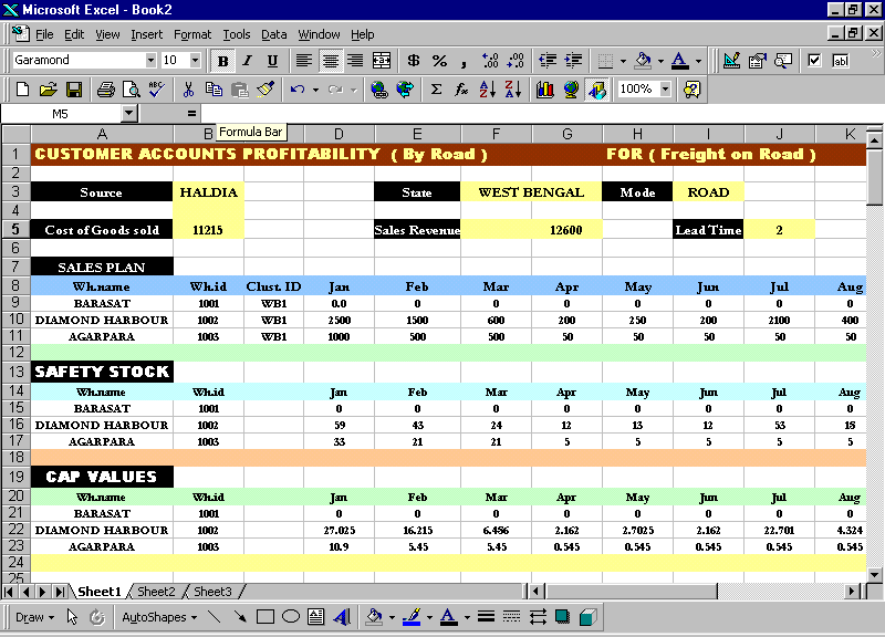
The lead-time is 2 days, for Road option, and a Just-In-Time Supply, on demand, is assumed since trucks are easily available.
The CAP value is calculated using the following algorithm:
![]()
The Sales Revenue, Cost Of goods sold, and the Transportation and handling Costs are per ton values and are provided. The net CAP serve as an input to the Mode Selection Module.
4.5.3 CAP By Railways INDIRECT
The Fertilizers reach the Rake-Head through the Railways. In the Indirect option through Rail, there is a Buffer warehouse at the Rake point, and the Non-Rake Point demands are met Just-In-Time from the Buffer Inventory.
The input to this algorithm is again the Sales Plan. The cumulative demand of the cluster is considered, and based on the requirements, the Amount ordered is calculated. The Amount ordered should always be a multiple of 2000, since a Rake carries 2000 tons only. Since no backlog of orders is considered, there is always some balance inventory left. Based on the Demand and the Lead-Time, the Safety Stock is calculated using the same algorithm:

Figure 4.4 CAP calculations Rail-INDIRECT #indirect.xls
It is assumed that the Fertilizers are sold at a uniform rate throughout the month, in the warehouses. The Inventory Held is therefore the sum of the Average inventory in a month and the safety stock and the Inventory carried to the next month.
![]()
The CAP Calculation, without Inventory follows the same algorithm as by Road, but Rental Costs, Inventory Holding Costs etc. come into play when Inventory is considered.
The CAP formulas, with and without Inventory are as follows:
CAPWithout Inventory = Demand * (RevenueSales - CostOfGoodsSold - CostTransportation - CostHandling
)CAPWith Inventory = CAPWithout Inventory - (Inventory * {CostInventory Holding + [CostRental/0.16]})
In the above expression, 0.16 represents space requirements in m2 per ton and the Rental Cost is in m2 per month.
The CAP values serve as an input to the Mode Selection Module.
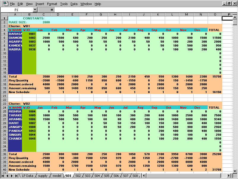
4.5.4 CAP by Railways DIRECT
In the Direct Option, the Supply received at the Rake head is at once distributed to the other Warehouses in the Cluster. Weights are assigned to the cluster members, depending on their demands. Later, the supply amount to individual Warehouses from the Rakes received is based on these weights.
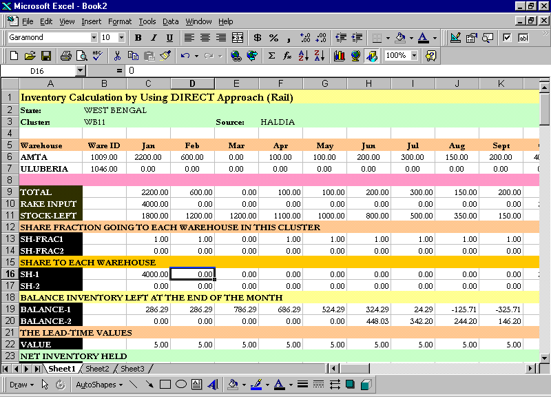
Figure 4.5.1 CAP calculations Rail-DIRECT #direct.xls
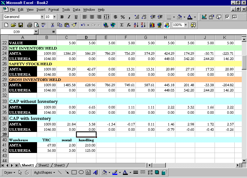
Figure 4.5.2 CAP calculations Rail-DIRECT #direct.xls
The Safety Stock and CAP algorithms are the same, the only difference is in the Inventory Holding, the Rentals paid, the Storage Space used and the Handling Costs. The screen shots above show a typical Cluster's CAP being calculated. The CAP values serve as inputs to the next module that we discuss, i.e. The Mode Selection Module.
The following Figure shows the Direct and Indirect Rail Mode options in details.
Figure 4.6 Direct and Indirect Options for Supply through Rail
4.6 The Mode Selection and Allocation of Warehouses to Plants Module
In the Mode Selection module, all the three options, i.e. Road, Rail - Direct and Indirect are evaluated based on their CAP values, and the best option is selected. The CAP per ton for the option giving the Maximum CAP value serves as the input for the LP coefficient in the Objective Function.
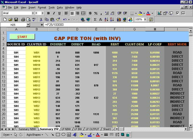
Figure 4.7 Selection Of Best mode by comparing CAP # lpcoeff.xls
The above sheet displays the various sources supplying the Warehouses in all the three modes and the CAPS associated with each mode, and finally the best mode to be considered for that particular combination of Source and Destination.
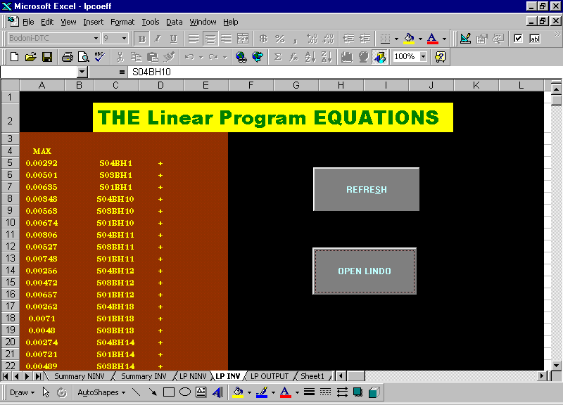
The LP Objective Functions and Constraints are generated from the data of this sheet. The LP formulation is as follows:
Z = S
iSubject to,
Si Xij = Dij
Sj Xij <= PI
Where,
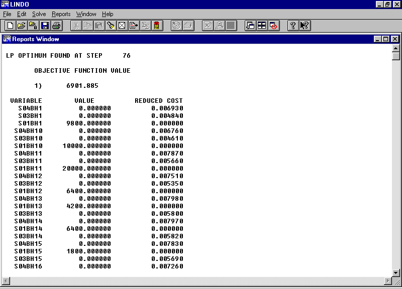
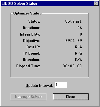
The Equations are generated in the Excel Sheets which triggers the optimization software LINDO, and a typical solution of the LP is as follows:
Figure 4.8 Objective Function Generation and solving the model using LINDO
4.7 The Vehicle Scheduling Module
The vehicle-scheduling module takes the Linear Programming solution as input and generates the schedules of trucks, rakes and ships. The following screen shows the allotment of fertilizers from sources to clusters, obtained from the database. This sheet is used as the basis of generating schedule. When the user presses ‘Generate Schedule’ button, the schedule generation starts.
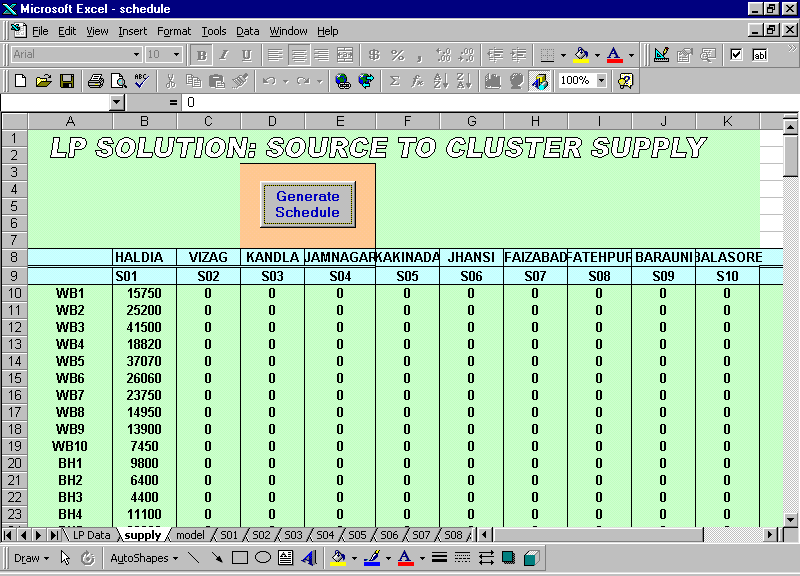
Figure 4.9 Schedule Generation from LP Solution # schedule_lp.xls
The algorithm for generating schedule is similar to that of determining CAP through direct or indirect mode. Here also a Model calculation sheet exists, and it gets copied subsequently as new clusters are added. Clusters are added in the page corresponding to their source. The calculations are automatically done by the embedded formulae in the excel sheet, and the results are tabulated in a summary page.
4.8 The Dynamic Scheduling of Dispatch Module
This module is aimed towards carrying out Sensitivity Analysis on the Schedule derived from the LP Solution. The analysis is carried out in three ways -
We will discuss these topics in the following section.
4.8.1 SPLIT - NO SPLIT Analysis
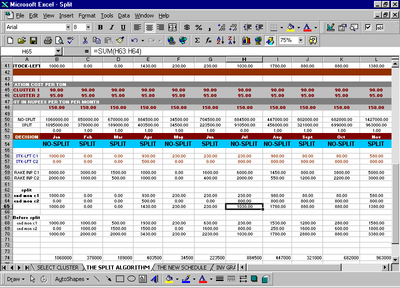
The Split Option means that the demands of 2 adjacent clusters can be met together, rather than treating them as separate entities. Indian Railways restricts Rake splitting to a maximum of 2 Rake points, i.e. part-rake can be supplied to 2 consecutive rake points, provided the distance between them is not very high and for this facility they charge 5% higher freight. Hence, though Splitting reduces Inventory Costs, it increases Freight Charges on the other side. This option is highly meaningful when the two clusters (to be clubbed) have very less demands, and it is more advisable to bring a single rake for both the clusters. The Inventory
and Transportation Cost calculations are the same, the only difference being that the total demand of both the clusters are considered together. The Inventory and Transportation Costs for a Warehouse pair is calculated for a particular month using both the Split and Non Split options, and the option giving minimum cost is preferred.
The Results show the months in which the cluster pair should switch to the SPLIT mode. Based on the results, the model also prepares a new revised schedule. Details on the Results are shown in the later chapters.
4.8.2 Schedule Sensitivity Analysis
The production of DAP in Haldia is constant (60000 Tons), but the demand pattern of the Warehouses supplied by Haldia (as from the LP Solution) is varying, showing a typical sinusoidal trend of very less demands in off-season and high demands in the peak season. Owing to this, the excess production has to be stocked at Haldia. The constraints to this idea are the limited storage space in Haldia and the high Inventory Holding charges. Thus it is necessary to transport the excess production during off-season to Warehouses that have high Demands during the later periods. Preferences are given to Warehouses that have low Rental Charges.
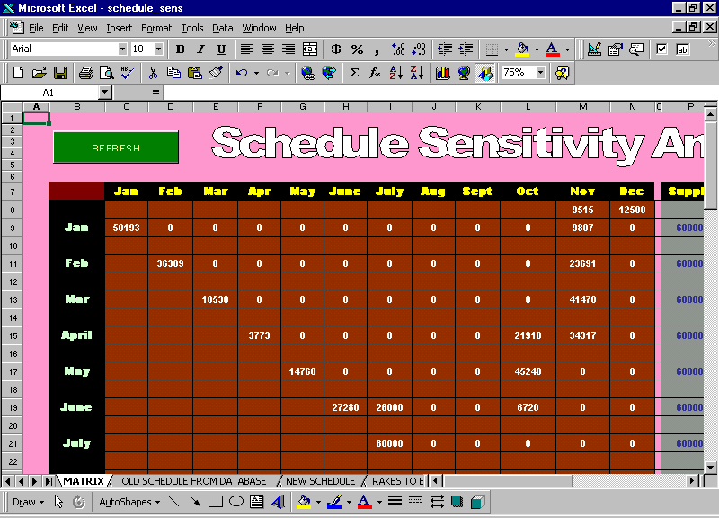
As an example of the algorithm, November has a demand of 178800 tons. Since only 60000 tons are produced in November, the rest has to be supplied from other months, where demand is lesser than the production. As shown below, the algorithm suggests that 9807 tons should be supplied from January production, 23691 tons from February, 41470 from March and 34317 from April. All these added up with the 60000 tons produced in November equals 178800 tons. Hence it is proposed that the excess productions of January, February, March and April, should be shipped to the Warehouses having high demands in November, with preference given to Warehouses having lower Rentals.
Figure 4.11 Triangular Matrix to determine distribution of excess Production in certain months # schedule_sens.xls
Based on this, a new Schedule is designed. We will discuss the results in the later chapters.
4.8.3 RUN-OUT TIME Analysis
ROT or Run-Out Time is defined as the ratio of present inventory less safety stock and present demand. Mathematically,
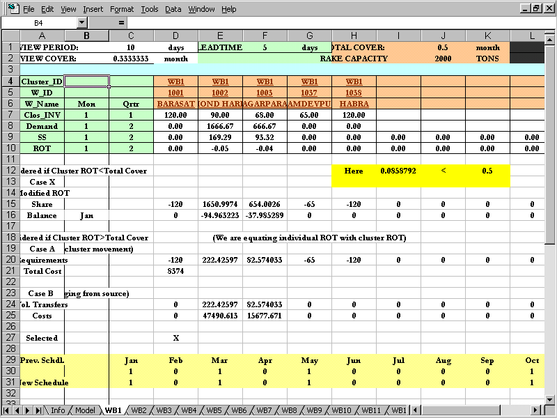
Figure 4.12 ROT Calculation Sheet # rot.xls
Inventory on hand – Safety Stock
ROT= -----------------------------------------------------
Demand for next period
ROT figures give an indication about how many days more the present stock will last given the demand pattern. ROT figures are calculated for individual warehouses as well as the cluster as a whole. We consider three cases that may arise:
Total cover is total of leadtime and review period converted into months.
(Total cover= (Leadtime + review period)/30 )
If cluster ROT is less than total cover, that indicates that the cluster will run out of stock before the ending of this cover period, i.e. demand during leadtime will exceed the stock. The only alternative here is to schedule a supply immediately.
Cluster ROT here is more than total cover period, which means no extra supply is necessary in the cluster. But the individual warehouse ROT’s may still be a mixture of positive and negative, indicating that in some warehouses stock will be left, whereas in others there will be a stock-out. There are two possible strategies that can be deployed.
We use the transportation algorithm to find out an optimal redistribution plan of stocks between warehouses (shown as case A in fig 4.14). The plan is shown in Fig. 4.14. The warehouses having negative requirements in row 20 acts as sources and those having positive requirements acts as destination. The per unit transportation cost between each pair of warehouses are obtained from the database. The algorithm used is lowest cost method for feasible solution.
This option (shown as case B in fig 4.14) suggests that the small shortfall of stock can be compensated by directly ordering to the source for a few trucks.
The cost-effective option of these two cases is chosen finally, and the schedule is dynamically updated to reflect these changes.

Figure 4.13 Revised Schedule Generation # rot.xls
4.9 The Warehouse Capacity Determination Module
After the LP optimization, followed by Sensitivity Analysis through various approaches, we have the Best combination of which Source should supply to which Warehouse, the Mode to be adopted and the Maximum, Average Inventories and Safety Stocks that it will need to hold over a month. Based on this we can make an estimate for the Average and Maximum Warehouse Space necessary at a particular Warehouse.
4.10 The Performance Measurement Module
While the Optimization and post-optimization Analysis is done by the DSS, a lot of assumptions are considered, like
Hence there always remains a discrepancy between the Results from the DSS and the actual data from the Warehouses. The Performance of the DSS can be measured through this discrepancy. The more the discrepancy, the lesser is the Performance Level of the DSS. The ways by which the Performance is measured are:
4.11 Conclusion
In all these modules, there is a Model sheet that gets replicated as new Clusters are added to the sheet. Visual Basic programs remain at the back end of the Excel sheets, where the reports are generated. All the Screen shot figures that are shown in this chapter are sheets showing intermediate calculations, however every module has a final sheet that gets prepared automatically, once calculations are done. So the user doesn't need to go through these intermediate sheets, unless he wants to analyze the final sheet results in a micro level or when he wants to change the algorithms itself.
The DSS-Model Base is made flexible, so that the discrepancy of the calculated data and real data is less, however there remains a scope of further generalizing the model, so that it exactly replicates the Real Life System. However, the unpredictable dynamics of Real Life Systems are a big constraint.